1 Intro

1.1 np.logspace

logspace可以创建等比数列.

In [19]: np.logspace(1, 2, 10)
Out[19]::
array([  10.        ,   12.91549665,   16.68100537,   21.5443469 ,
         27.82559402,   35.93813664,   46.41588834,   59.94842503,
         77.42636827,  100.        ])

1.2 np.linspace

linspace函数通过指定起始值、终止值和元素个数来创建数组，缺省包括终止值.

In [18]: np.linspace(1, 10, 10, endpoint=False)
Out[18]: array([ 1. ,  1.9,  2.8,  3.7,  4.6,  5.5,  6.4,  7.3,  8.2,  9.1])

1.3 slice

a = np.arange(10)
print a
# # 获取某个元素
print a[3]
# # # 切片[3,6)，左闭右开
print a[3:6]
# # # 省略开始下标，表示从0开始
print a[:5]
# # # 下标为负表示从后向前数
print a[3:]
# # # 步长为2
print a[1:9:2]
# # # 步长为-1，即翻转

2 Linear Regression with Multiple Variables

Gradient Descent:

Taking the derivative (the tangential line to a function) of our cost function. The slope of the tangent is the derivative at that point and it will give us a direction to move towards. We make steps down the cost function in the direction with the steepest descent. The size of each step is determined by the parameter α, which is called the learning rate.

Algorithm:

\[\Theta_j = \Theta_j + \Alpha\Derivative{J(\Theta_0,\Theta_1)}\] Update simutaneously: \[Temp_0 := \Theta_0 - \Alpha\Derivative{J(\Theta_0,\Theta_1)} \] \[Temp_1 := \Theta_1 - \Alpha\Derivative{J(\Theta_0,\Theta_1)} \]

normalization

\[\theta_0 = \theta_0 - \alpha\partial{J(\theta)}{\theta}\]

3 Polynomial regression

4 Taylor expansion:

taylor_expansion

# -*- coding: utf-8 -*-
import numpy as np
import math
import pprint


def cal_e_small(x):
    n = 10
    f = np.arange(1, n+1).cumprod()
    b = np.array([x]*n).cumprod()
    return np.sum(b/f) + 1


def cal_e(x):
    reverse = False
    if x < 0:
        x = -x
        reverse = True
    ln2 = 0.69314718055994529
    c = x / ln2
    a = int(c + 0.5)
    b = x - a * ln2
    y = (2 ** a) * cal_e_small(b)
    if reverse:
        return 1 / y
    return y


t1 = np.linspace(-2, 0, 10, endpoint=False)
t2 = np.linspace(0, 2, 20)
t = np.concatenate((t1, t2))
print(t)
y = np.empty_like(t)
for i, x in enumerate(t):
    y[i] = cal_e(x)
    print('e^', x, ' = ', y[i], ', appx = \t', math.exp(x))

e^ -2.0  =  0.135335283237 , appx =    0.1353352832366127
e^ -1.8  =  0.165298888222 , appx =    0.16529888822158653
e^ -1.6  =  0.201896517995 , appx =    0.20189651799465538
e^ -1.4  =  0.246596963942 , appx =    0.2465969639416065
e^ -1.2  =  0.301194211912 , appx =    0.30119421191220214
e^ -1.0  =  0.367879441171 , appx =    0.36787944117144233
e^ -0.8  =  0.449328964117 , appx =    0.4493289641172217
e^ -0.6  =  0.548811636094 , appx =    0.5488116360940265
e^ -0.4  =  0.670320046036 , appx =    0.6703200460356393
e^ -0.2  =  0.818730753078 , appx =    0.8187307530779819
e^ 0.0  =  1.0 , appx =    1.0
e^ 0.105263157895  =  1.11100294108 , appx =   1.1110029410844708
e^ 0.210526315789  =  1.2343275351 , appx =    1.2343275350983443
e^ 0.315789473684  =  1.37134152176 , appx =   1.3713415217558058
e^ 0.421052631579  =  1.5235644639 , appx =    1.523564463901954
e^ 0.526315789474  =  1.69268460033 , appx =   1.692684600326856
e^ 0.631578947368  =  1.88057756929 , appx =   1.8805775692915292
e^ 0.736842105263  =  2.08932721042 , appx =   2.089327210420374
e^ 0.842105263158  =  2.32124867566 , appx =   2.3212486756648487
e^ 0.947368421053  =  2.57891410565 , appx =   2.57891410565208
e^ 1.05263157895  =  2.86518115618 , appx =    2.8651811561836884
e^ 1.15789473684  =  3.18322469126 , appx =    3.1832246912598827
e^ 1.26315789474  =  3.53657199412 , appx =    3.5365719941224363
e^ 1.36842105263  =  3.92914188683 , appx =    3.929141886826998
e^ 1.47368421053  =  4.3652881922 , appx =   4.365288192202982
e^ 1.57894736842  =  4.84984802022 , appx =    4.849848020218827
e^ 1.68421052632  =  5.38819541428 , appx =    5.388195414275814
e^ 1.78947368421  =  5.9863009524 , appx =   5.986300952398287
e^ 1.89473684211  =  6.65079796433 , appx =    6.650797964331267
e^ 2.0  =  7.38905609893 , appx =    7.38905609893065

5 损失函数

\[\theta^*=arg min L(f(x,\theta), y)\]

Logitic loss
0/1 loss
Hinge loss

x = np.array(np.linspace(start=-2, stop=3, num=1001, dtype=np.float))
y_logit = np.log(1 + np.exp(-x)) / math.log(2)
y_boost = np.exp(-x)
y_01 = x < 0
y_hinge = 1.0 - x
y_hinge[y_hinge < 0] = 0
plt.plot(x, y_logit, 'r-', label='Logistic Loss', linewidth=2)
plt.plot(x, y_01, 'g-', label='0/1 Loss', linewidth=2)
plt.plot(x, y_hinge, 'b-', label='Hinge Loss', linewidth=2)
plt.plot(x, y_boost, 'm--', label='Adaboost Loss', linewidth=2)
plt.grid()
plt.legend(loc='upper right')
# plt.savefig('1.png')
plt.show()

6 重心插值

Cubic Spine
Barycentric Interpolator

from scipy.interpolate import BarycentricInterpolator
from scipy.interpolate import CubicSpline
rv = poisson(5)
x1 = a[1]
y1 = rv.pmf(x1)
itp = BarycentricInterpolator(x1, y1)  # 重心插值
x2 = np.linspace(x.min(), x.max(), 50)
y2 = itp(x2)
cs = scipy.interpolate.CubicSpline(x1, y1)       # 三次样条插值
plt.plot(x2, cs(x2), 'm--', linewidth=5, label='CubicSpine')           # 三次样条插值
plt.plot(x2, y2, 'g-', linewidth=3, label='BarycentricInterpolator')   # 重心插值
plt.plot(x1, y1, 'r-', linewidth=1, label='Actural Value')             # 原始值
plt.legend(loc='upper right')
plt.grid()
plt.show()

7 绘制三维图像

x, y = np.ogrid[-3:3:100j, -3:3:100j]
u = np.linspace(-3, 3, 101)
x, y = np.meshgrid(u, u)
z = x*y*np.exp(-(x**2 + y**2)/2) / math.sqrt(2*math.pi)
fig = plt.figure()
ax = fig.add_subplot(111, projection='3d')
ax.plot_surface(x, y, z, rstride=5, cstride=5, cmap=cm.coolwarm, linewidth=0.1)  #
ax.plot_surface(x, y, z, rstride=5, cstride=5, cmap=cm.Accent, linewidth=0.5)
plt.show()

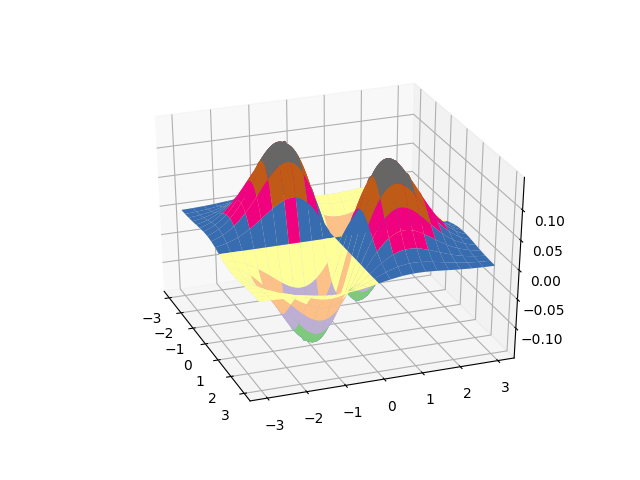
Figure 1: 3d plot

Table of Contents